
Completion requirements
Density Functions
Discrete Variables

The outcome of dice is a discrete variable because it has only outcomes in the range of 1 to 6 and values like 3.5, 5.2 are not possible [1, 5, 7, 12, 33, 35, 37, 39].
The dice has six possible outcomes and each of
these outcomes has a probability of 1/6. This probability is called mass
function (fig. 5.1):
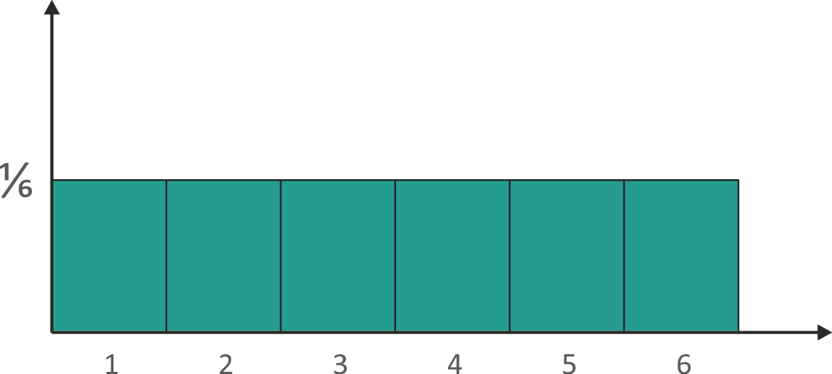
Fig. 5.1 Probability mass
function
The cumulative distribution function looks like this (Fig. 5.2):
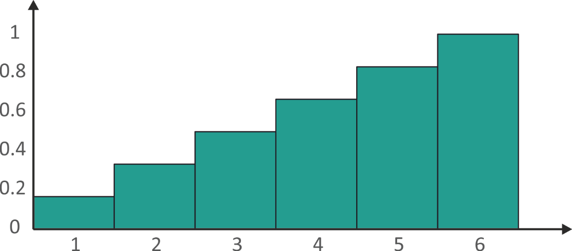
Fig. 5.2 Cumulative distribution function
The meaning of cumulative probability for 3 doesn’t represent the probability for outcome to be 3, but the probability the outcome to be 3 or less:
\( P(X \leq3 )=P(X=1 )+P(X=2 )+P(X=3 ) \) (5.1)
Graphical representation of above equation (Fig. 5.3):
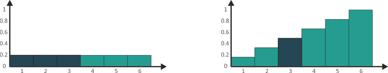
Fig. 5.3 Graphical representation of (5.1)
Continuous Variables
For example, the height of the students is a continuous variable. It can take an infinite number of values:
According to the measurement device the height of a student could be: 165 cm, 165.2 cm, 165.27 cm or even 165.2564 cm.
The probability density function for the height of students looks like (Fig. 5.4):
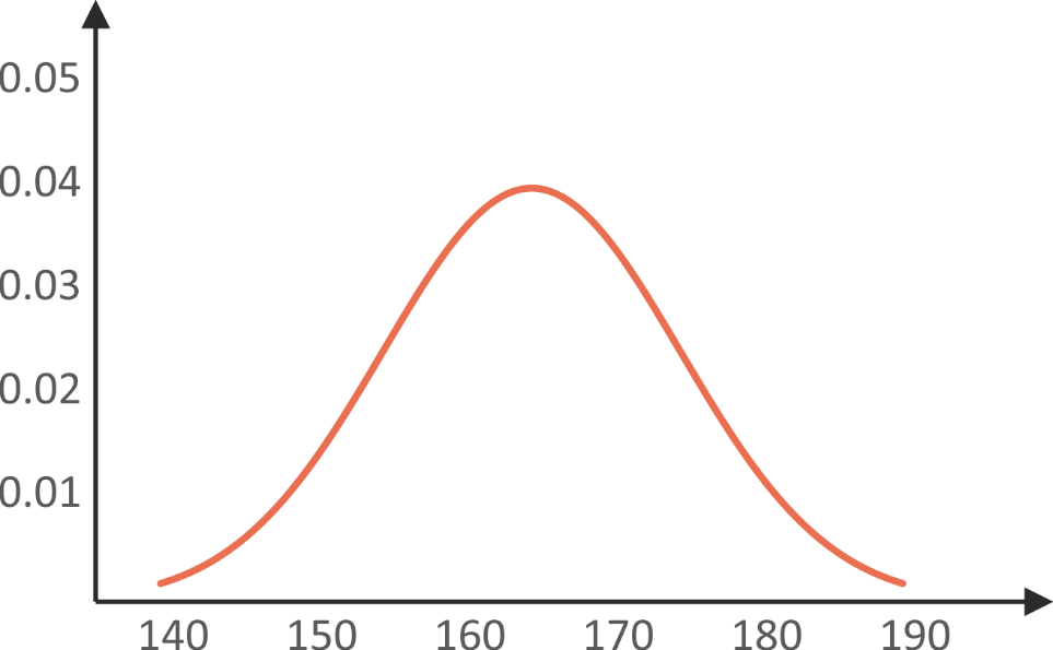
Fig. 5.4 Probability density function
From the above graphic we can see that the mean is 165 cm. This means the
height of most of the students is around 165 cm.
The cumulative distribution function for this case looks like this (Fig. 5.5):
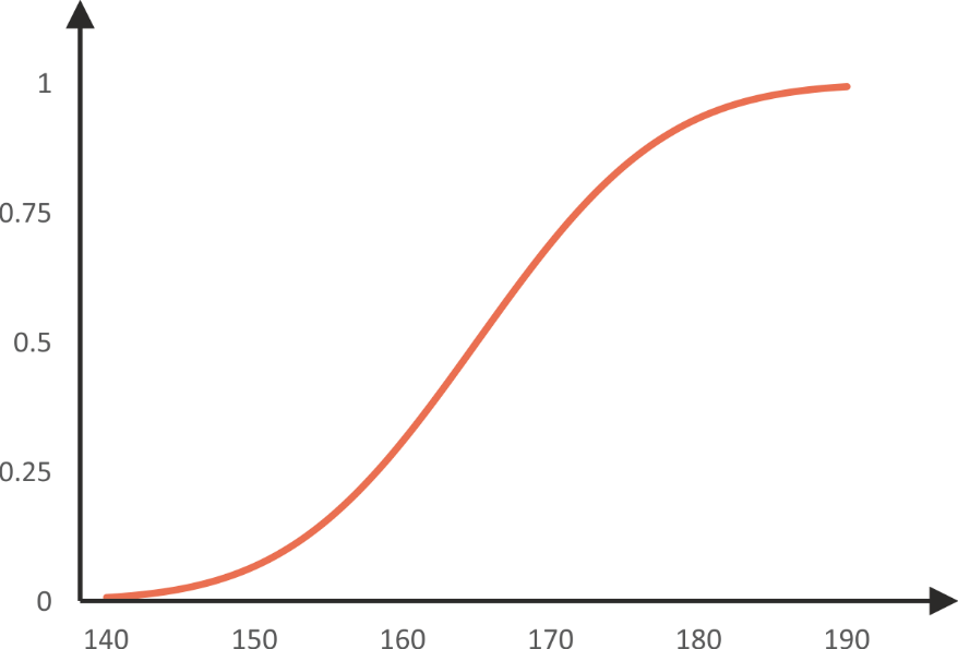
Fig. 5.5 Cumulative distribution function
Link between the probability density function and the cumulative distribution function
If we select the mean value (165 cm) on the probability density, we know that the proportion of the distribution on the left is 0.5. So, the orange region on the picture is 50% of the whole distribution (Fig. 5.6).
This is represented on the cumulative distribution function: at 165 it goes up to a value of 0.5. This means that 50% of distribution is elapsed at this point.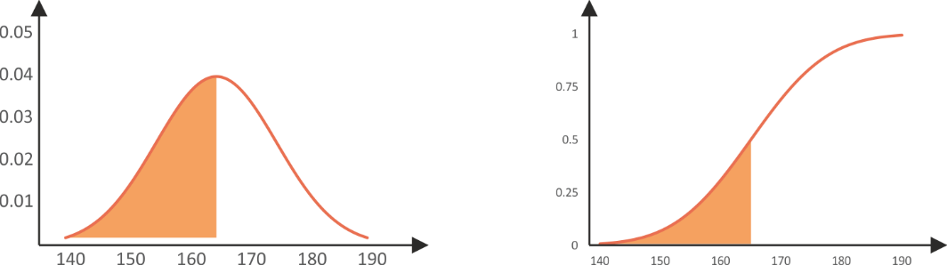
Fig. 5.6 Link between the probability density function and the cumulative distribution function