
Completion requirements
Control Charts for Variables
X̄ and R chart
When the result of the control is variable data, which is generated frequently and a sample less than 10 item is enough to represent the production the \( \bar{X}\ and\ R \) chart chart is recommended [4, 5, 7, 9, 16-20, 36].
Typically the \( \bar{X} \) chart is drawn above the \( R \) chart. The values of \( \bar{X} \) and \( R \) are represented on the \( y \) axis and the sequence of the subgroups through time is represented on the \( x \) axis.
Calculation of the average and range of each subgroup is done by the following formulas:
\( \bar{X}=\frac{X_1+X_2+...+X_n}{n} \) (9.1)
\( R=X_{max}+X_{min} \) (9.2)
where
\( X_1 \), \( X_2 \), \( ... \) - the individual values within the subgroup
\( n \) - subgroup
sample size
Calculation of the average range and the process average is done by the following formulas:
\( \bar{\bar{X}}=\frac{{\bar{X}}_1+{\bar{X}}_2+...+{\bar{X}}_k}{k} \) (9.3)
\( \bar{R}=\frac{R_1+R_2+...+R_k}{k} \) (9.4)
where
\( k \) - number
of subgroups
\( X_1 \), \( X_2 \), \( ... \) - are the averages of each subgroup
\( R_1 \), \( R_2 \), \( ... \) - are the ranges of each subgroup
Calculation of the control limits is done by the following formulas:
For the \( \bar{X} \) chart:
\( {UCL}_{\bar{X}}=\bar{\bar{X}}+A_2\bar{R} \) (9.5)
\( {LCL}_{\bar{X}}=\bar{\bar{X}}-A_2\bar{R} \) (9.6)
For the \( R \) chart:
\( {UCL}_R=D_4\bar{R} \) (9.7)
\( {LCL}_R=D_3\bar{R} \) (9.8)
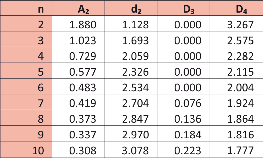
Fig. 9.3 Constants for calculation of the control limits
Example
Create a\( \bar{X}\ and\ R \) control chart for the linear density of cotton sliver. The sampling plan is used to select four units every one hour. The operator measures the linear density and record the value it in Nm (See Table 9.1). For facilitation, the values have been multiplied by 1000 i.e., when the measured value has been 0.251, the recorded value is 251.
Table 9.1 Units linear density
|
Sample |
Unit 1 |
Unit 2 |
Unit 3 |
Unit 4 |
|
|
1 |
272 |
252 |
245 |
255 |
|
|
2 |
274 |
254 |
272 |
247 |
|
|
3 |
264 |
251 |
257 |
255 |
|
|
4 |
263 |
248 |
244 |
269 |
|
|
5 |
269 |
251 |
273 |
244 |
|
|
6 |
263 |
273 |
274 |
272 |
|
|
7 |
258 |
266 |
266 |
247 |
|
|
8 |
252 |
276 |
273 |
272 |
|
|
9 |
258 |
267 |
275 |
250 |
|
|
10 |
261 |
254 |
256 |
261 |
|
|
11 |
252 |
250 |
254 |
246 |
|
|
12 |
270 |
247 |
249 |
254 |
First, we calculate the average and range of each subgroup. Te results are presented in Table 9.2:
Table 9.2 Average and range of each subgroup
|
x1 |
256.00 |
R1 |
27 |
|
x2 |
261.75 |
R2 |
27 |
|
x3 |
256.75 |
R3 |
13 |
|
x4 |
256.00 |
R4 |
25 |
|
x5 |
259.25 |
R5 |
29 |
|
x6 |
270.50 |
R6 |
11 |
|
x7 |
259.25 |
R7 |
19 |
|
x8 |
268.25 |
R8 |
24 |
|
x9 |
262.50 |
R9 |
25 |
|
x10 |
258.00 |
R10 |
7 |
|
x11 |
250.50 |
R11 |
8 |
|
x12 |
255.00 |
R12 |
23 |
The next step is the calculation of the average range and the process average using formulas (9.3) and (9.4):
\( \bar{\bar{X}}=\frac{256+261.75+...+255}{12}=259.48 \)
\( R=\frac{27+27+...+23}{12}=19.83 \)
Finally, we plug the values in the formulas (9.5), (9.6), (9.7) and (9.8) for the control limits:
\( {UCL}_{\bar{X}}=259.48+0.729*19.83=273.94 \)
\( {LCL}_{\bar{X}}=259.48-0.729*19.83=245.02 \)
\( {UCL}_R=2.282*19.83=45.26 \)
\( {LCL}_R=0*19.83=0 \)
According to the calculations, we can construct the \( \bar{X}\ and\ R \) control chart (Fig. 9.4):
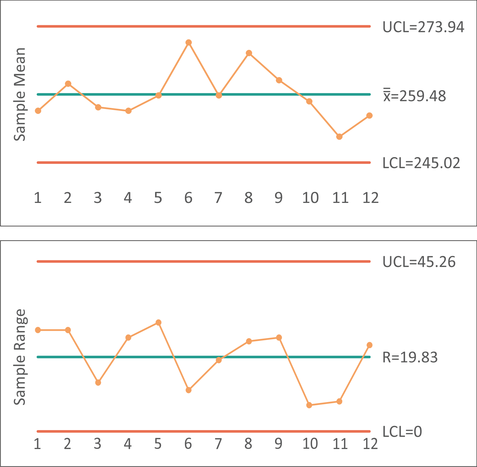
Fig. 9.4 \( \bar{X}\ and\ R \) control chart
X̄ and s chart
\( \bar{X}\ and\ s \) is used when the result of the control is variable data, and a sample size group is more than 10. \( \bar{X}\ and\ s \) is very similar to an \( \bar{X}\ and\ R \), but the subgroup variation is estimated by the standard deviation, instead of the range [4, 5, 7, 9, 16-20, 36].
Calculation of the average and standard deviation of each subgroup is done by the following formulas:
\( \bar{X}=\frac{X_1+X_2+...+X_n}{n} \) (9.9)
\( s=\sqrt{\frac{X_1^2+X_2^2+...-n{\bar{X}}_n^2}{n-1}} \) (9.10)
\( X_1 \), \( X_2 \), \( ... \) - are the individual values within the subgroup
\( \bar{X} \) - the sample mean
\( n \) - the subgroup size
Calculation of the average standard deviation and the process average is done by the following formulas:
\( \bar{\bar{X}}=\frac{{\bar{X}}_1+{\bar{X}}_2+...+{\bar{X}}_k}{k} \) (9.11)
\( s=\frac{s_1+s_2+...+s_k}{k} \) (9.12)
where
\( k \)
\( \bar{X}_1 \), \( \bar{X}_2 \), \( ... \) - are
the averages of each subgroup
Calculation of the control limits is done by the following formula:
\( {UCL}_{\bar{X}}=\bar{\bar{X}}+A_3\bar{s} \) (9.13)
\( {LCL}_{\bar{X}}=\bar{\bar{X}}-A_3\bar{s} \) (9.14)
\( {UCL}_S=B_4\bar{s} \) (9.15)
\( {LCL}_S=B_3\bar{s} \) (9.16)
Example
If instead of taking samples consisting of four units as in the x/r example, the organization decided to take samples consisting of 12 units. A s chart should be used instead of R.
Again, the first step is the calculation of the average and standard deviation of each subgroup (Table 9.3):
Table 9.3 Average and standard
deviation of each subgroup
|
x1 |
256.17 |
s1 |
7.44 |
|
x2 |
259.42 |
s2 |
7.03 |
|
x3 |
261.75 |
s3 |
9.26 |
|
x4 |
262.08 |
s4 |
11.19 |
|
x5 |
264.25 |
s5 |
9.32 |
|
x6 |
258.50 |
s6 |
9.26 |
|
x7 |
259.75 |
s7 |
8.32 |
|
x8 |
261.25 |
s8 |
10.04 |
|
x9 |
258.00 |
s9 |
10.41 |
|
x10 |
259.42 |
s10 |
11.45 |
|
x11 |
258.75 |
s11 |
10.60 |
|
x12 |
255.25 |
s12 |
8.90 |
The next step is the calculation of the average standard deviation and the process average using formulas (9.11) and (9.12):
\( \bar{\bar{X}}=\frac{256.17+259.42+...+255.25}{12}=259.55 \)
\( s=\frac{7.44+7.03+...+8.90}{12}=9.44 \)
Finally, we plug the values in the formulas (9.13), (9.14), (9.15) and (9.16) for the control limits:
\( {UCL}_{\bar{X}}=259.55+0.8859*9.44=267.91 \)
\( {LCL}_{\bar{X}}=259.55+0.8859*9.44=251.19 \)
\( {UCL}_s=1.6465*9.44=15.54 \)
\( {LCL}_s=0.3535*9.44=3.34 \)
According to the calculations, we can construct the \( \bar{X}\ and\ s \) control chart:
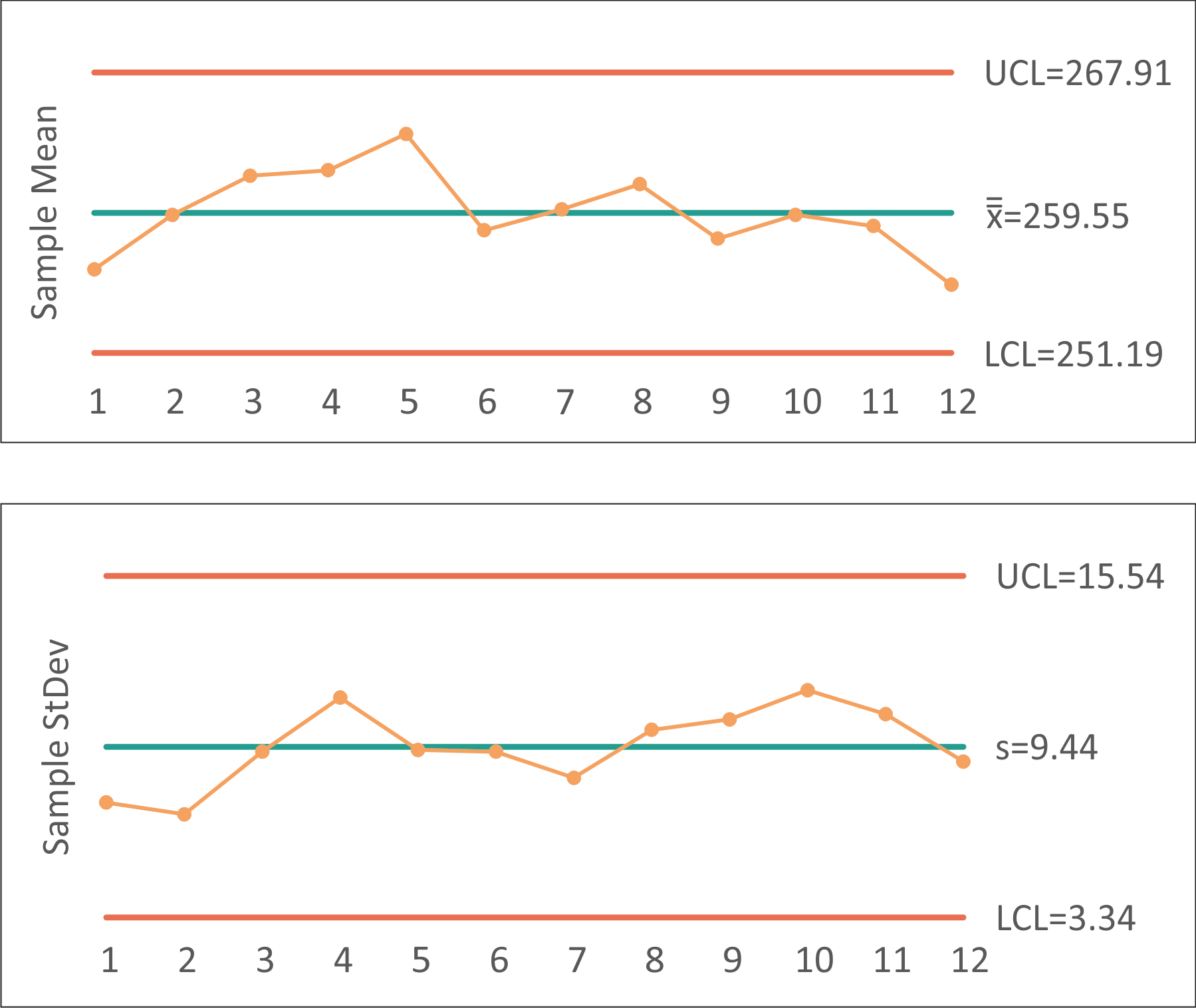
Fig. 9.5 \( \bar{X}\ and\ s \) control chart
I-MR chart
In some cases, the measurements are too expensive (e.g., a destructive test) or the output is relatively homogenous the chartfor individuals and moving range (\( I-MR \) chart) is recommended [4, 5, 7, 9, 16-20, 36].
Formulas for the construction of the charts are:
\( \bar{X}=\frac{X_1+X_2+...+X_k}{k} \) (9.17)
\( \bar{MR}=\frac{\sum\left|X_i-X_{i-1}\right|}{k-1} \) (9.18)
where
\( X_1 \), \( X_2 \), \( ... \) - are the individual values
\( k \) - number
of observations
\( \bar{X} \) - the
center line for the \( I \) chart
Calculation of the control limits is done by the following
formulas
\( {UCL}_X=\bar{X}+E_2\bar{MR} \) (9.19)
\( {LCL}_X=\bar{X}-E_2\bar{MR} \) (9.20)
\( {UCL}_{MR}=D_4\bar{MR} \) (9.21)
\( {LCL}_{MR}=D_3\bar{MR} \) (9.22)
Example
A quality engineer monitors the manufacture of cotton sliver and wants to assess whether the process is in control. The engineer measures the linear density of 25 consecutive batches.
The data from the measurement is in Table 9.4:
Table 9.4 Values of the linear density
|
n |
1 |
2 |
3 |
4 |
5 |
6 |
7 |
8 |
9 |
10 |
11 |
12 |
13 |
|
Value |
271 |
255 |
248 |
248 |
272 |
247 |
268 |
260 |
273 |
248 |
251 |
267 |
254 |
|
n |
14 |
15 |
16 |
17 |
18 |
19 |
20 |
21 |
22 |
23 |
24 |
25 |
|
|
Value |
260 |
261 |
258 |
251 |
256 |
252 |
249 |
266 |
268 |
266 |
266 |
261 |
|
The first step is the calculation of the values for the \( MR \) chart using formula (9.18). The results are in Table. 9.5:
Table 9.5 Values for the \( MR \) chart
|
No |
\( I \) Chart |
\( MR \) Chart |
|
1 |
271 |
|
|
2 |
255 |
16 |
|
3 |
248 |
7 |
|
4 |
248 |
0 |
|
5 |
272 |
24 |
|
6 |
247 |
25 |
|
7 |
268 |
21 |
|
8 |
260 |
8 |
|
9 |
273 |
13 |
|
10 |
248 |
25 |
|
11 |
251 |
3 |
|
12 |
267 |
16 |
|
13 |
254 |
13 |
|
14 |
260 |
6 |
|
15 |
261 |
1 |
|
16 |
258 |
3 |
|
17 |
251 |
7 |
|
18 |
256 |
5 |
|
19 |
252 |
4 |
|
20 |
249 |
3 |
|
21 |
266 |
17 |
|
22 |
268 |
2 |
|
23 |
266 |
2 |
|
24 |
266 |
0 |
|
25 |
261 |
5 |
The center lines are:
\( \bar{X}=259.04 \)
\( \bar{MR}=9.42 \)
The control limits are calculated by plugging the values in formulas (9.19), (9.20), (9.21) and (9.22):
\( {UCL}_X=259.04+2.66*30.79=284.09 \)
\( {LCL}_X=259.04+2.66*30.79=233.99 \)
\( {UCL}_{MR}=3.27*9.42=30.79 \)
\( {LCL}_{MR}=0*9.42=0 \)
Now we are able to construct the chart (Fig. 9.6):
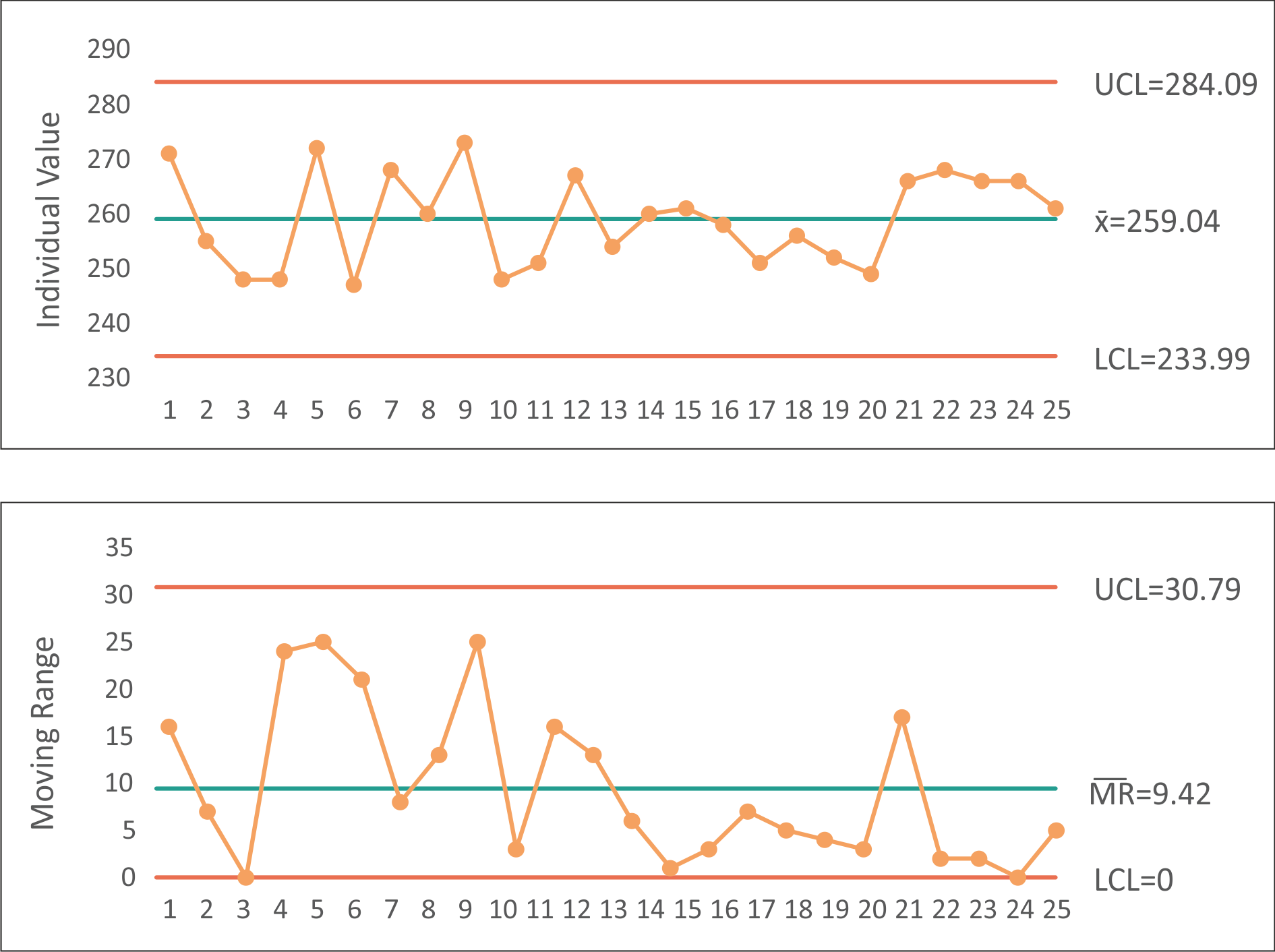
Fig. 9.6 \( I-MR \) chart